The Math Behind Shazam: How Your Phone Recognizes Any Song in Seconds

You're sitting in a café. A song drifts through the speakers — you know you know it, but the name is completely gone. You pull out your phone, tap Shazam, and within five seconds, it tells you the exact track, artist, and album. No lyrics typed, no humming, no searching. Just raw audio captured through a noisy room.

This feels like magic. It isn't. Underneath that tap lies one of the most elegant algorithms in applied mathematics — a system built from signal processing, combinatorial hashing, and probabilistic matching that works reliably even with background noise, poor microphones, and truncated recordings. This is how it works.

A Brief History: From a Pub Epiphany to Apple's Acquisition

The story begins in 1999, when Chris Barton — an MBA student at UC Berkeley — found himself frustrated in a London bar, unable to identify a song playing over the speakers. He had a simple but radical idea: what if a phone could do it for you, just from the sound in the air?

Barton co-founded Shazam Entertainment Ltd alongside Philip Inghelbrecht and Dhiraj Mukherjee. The critical hire came when Professor Julius Smith of Stanford pointed them toward Avery Wang, a PhD in digital signal processing. Wang's initial verdict on the project was blunt: "It's impossible." The challenges were substantial — the system needed to recognize music in real time, through ambient noise, at a scale of millions of songs, over the notoriously low-quality audio channels of early mobile phones.

Wang nearly quit. Then, in June 2000, he cracked it, inventing the fingerprinting system that powers Shazam to this day.

In 2002, the service launched in the UK — not as an app, but as a four-digit phone number (2580). Users would call the number, hold their phone up to a speaker, and receive a text message identifying the song. The choice of 2580 was intentional: these keys are arranged in a straight vertical line down the middle of an old mobile phone keypad, making it incredibly easy to dial while on the move in a loud pub. The database at launch held one million songs and took around 15 seconds to respond.

When Apple launched the App Store in 2008, everything changed overnight. Shazam was one of the first apps available, and friction vanished entirely. By 2022, the app had been downloaded over 2 billion times. Apple formally announced its agreement to acquire Shazam in December 2017, officially closing the deal in September 2018 for an estimated $400 million.

The algorithm published by Avery Wang in his landmark 2003 paper — "An Industrial-Strength Audio Search Algorithm" — remains the foundational architecture of the system today.

The Core Problem: Why Audio Recognition Is Hard

Before examining the solution, it's worth understanding precisely why recognizing a song from a noisy 10-second sample is a difficult computational problem.

The challenge is threefold:

Scale. Shazam's database contains hundreds of millions of songs. A fingerprint from a sample must be matched against this entire catalog within seconds.
Noise. The captured audio contains background chatter, room acoustics, low-quality microphone compression, and transmission artifacts — none of which are present in the pristine studio recording in the database.
Temporal offset. The sample could be taken from any point in the song — the opening, the bridge, the outro — so matching cannot rely on absolute position within the track.

A naive approach — comparing raw waveforms — would fail all three tests instantly. The waveform of your recorded sample and the waveform of the studio track are simply too different to correlate directly. A smarter representation of the audio is needed.

Step 1: Capturing and Optimizing the Signal

When you tap Shazam, the app records a 5–10 second audio sample through your device's microphone. This analog sound — a continuous pressure wave traveling through air — is converted into a digital signal through a process called Analog-to-Digital Conversion (ADC).

While standard high-fidelity audio is typically recorded at 44,100 samples per second (44.1 kHz), Shazam employs an ingenious downsampling and optimization strategy to save memory and processing power. The incoming audio is downsampled to 8 kHz (or sometimes 11 kHz) and converted from stereo to a single mono channel before any further mathematical processing occurs.

Why does this optimization work so well? Human hearing extends up to 20 kHz, but the vast majority of the unique "energetic" characteristics that distinguish popular music—such as vocals, percussion transients, and dominant harmonic structures—lie comfortably below 4 kHz. According to the Nyquist-Shannon sampling theorem, a sampling rate of 8 kHz is mathematically sufficient to perfectly capture and reconstruct all frequencies up to 4 kHz. This optimization step drastically compresses the volume of data the algorithm must process every second without losing the vital features needed for identification.

Step 2: The Fourier Transform — Decomposing Sound into Frequencies

The foundational mathematical tool that makes Shazam possible is the Discrete Fourier Transform (DFT), implemented in practice via the computationally optimized Fast Fourier Transform (FFT).

The DFT takes a time-domain signal — a sequence of amplitudes — and decomposes it into its constituent frequency components. In plain terms: it tells you not how loud the sound is at any moment, but which frequencies are present, and at what intensity.

Mathematically, the DFT of a signal $x[n]$ of length $N$ is beautifully expressed in LaTeX format as:

$X[k] = \sum_{n=0}^{N-1} x[n] \cdot e^{-j\frac{2\pi}{N}kn}$

Where:

$x[n]$ is the input time-domain signal (amplitude at sample $n$ )
$X[k]$ is the complex frequency-domain output at frequency bin $k$
$e^{-j\frac{2\pi}{N}kn}$ is a complex exponential representing a rotating unit vector
$|X[k]|$ gives the magnitude (amplitude) at frequency $k$

The FFT computes this transform in $O(N \log N)$ time rather than the naive $O(N^2)$ , making real-time audio processing highly feasible on consumer hardware.

The problem with a single FFT over the entire sample is that music is not stationary — frequencies change dynamically over time. A single FFT would tell you that a guitar, piano, and bass are all present somewhere, but completely lose the temporal context of when each note occurs.

Step 3: The Short-Time Fourier Transform and the Spectrogram

To capture how frequencies evolve over time, Shazam applies the Short-Time Fourier Transform (STFT). Instead of running one massive FFT over the full clip, the algorithm slides a small analysis window — typically 10–30 milliseconds wide — along the signal and computes an FFT at each discrete interval.

The result is a 2D representation:

Horizontal axis: Time (each window position)
Vertical axis: Frequency (each FFT frequency bin)
Color/intensity: Amplitude (magnitude of that frequency at that moment)

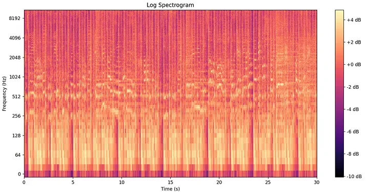
This 2D structure is called a spectrogram, and it serves as the core landscape for fingerprinting.

A visual spectrogram of an audio signal showing frequency content across time as a heatmap

To prevent an artifact known as spectral leakage—where energy from one sharp frequency bin "bleeds" into neighboring bins due to the abrupt cutoffs of a rectangular window—the STFT applies a Hamming window function. This smooth bell curve tapers the edges of each analysis frame. The Hamming window $w[n]$ is defined mathematically as:

$w[n] = 0.54 - 0.46 \cdot \cos\left(\frac{2\pi n}{N-1}\right)$

A spectrogram of a song captures its full acoustic fingerprint grid. However, comparing raw matrices across a database of millions of songs would still be computationally crippling. Further abstraction is required.

Step 4: The Constellation Map — Extracting Spectral Peaks

Here is where Avery Wang's central insight shines. Most of a spectrogram consists of background noise, reverb, and low-energy filler. The acoustically meaningful elements in music — the transient punch of a kick drum, the onset of a guitar chord, or the peak of a vocal melody — manifest as local maxima in the spectrogram. These are points that are more intense than all their immediate neighbors in both time and frequency.

Shazam's algorithm identifies these spectral peaks and discards everything else. A peak is a point $(t, f)$ whose magnitude $|X(t, f)|$ exceeds all neighbors within a defined local region on the 2D time-frequency grid.

This strips the dense spectrogram down to a sparse scatter plot of coordinate pairs. Because this scatter plot resembles stars in a night sky, it is formally known as a constellation map.

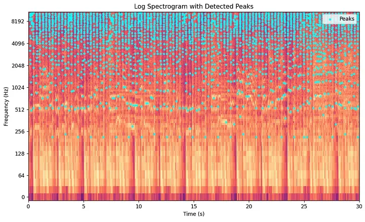
An annotated constellation map showing spectral peak coordinates scattered across a time-frequency grid

This step provides powerful noise resilience. Background chatter or low-quality speaker distortions distribute energy evenly and at lower levels across the spectrogram grid. They rarely generate the dominant, concentrated local peaks required to pass the thresholding step. The spectral peaks that survive are the acoustically strongest elements, allowing Shazam to work even in a chaotic bar. Furthermore, storing only peak coordinates instead of full spectrogram matrices compresses the required storage capacity by several orders of magnitude.

Step 5: Combinatorial Hashing — Turning Points into Fingerprints

A single isolated point on a constellation map carries very little entropy. A frequency of 1,400 Hz occurs across thousands of different tracks. What makes an audio signature highly distinct is its combinatorial relationship to surrounding points.

To unlock this specificity, Shazam’s algorithm pairs each anchor point with multiple target points falling within a predefined time-frequency "target zone" located ahead of it. For each unique anchor-target pair, it computes a compact, highly discriminative hash from three structural variables:

hash = (f_anchor, f_target, Δt)

Where:

f_anchor is the frequency of the anchor peak
f_target is the frequency of the target peak
Δt = t_target − t_anchor is the precise time delta between them

To maximize database performance at the processor level, Wang utilized an elegant bit-packing strategy to encode this entire triple into a single 32-bit unsigned integer (uint32):

Frequency of Anchor ( $f_A$ ): 9 bits (allocating 512 distinct frequency bins)
Frequency of Target ( $f_T$ ): 9 bits (allocating 512 distinct frequency bins)
Time Delta ( $\Delta t$ ): 14 bits
Total: $9 + 9 + 14 = 32$ bits

This 32-bit integer structure allows the system's database to perform lightning-fast, hardware-level equality lookups. These hashes are stored in a massive hash table, indexed by the hash value itself. Each entry maps directly to the corresponding track identification and the absolute timestamp where the anchor point occurred in the studio version:

hash → { track_id, t_anchor }

Because the hash only captures the relative time delta ( $\Delta t$ ) between the two peaks rather than an absolute timeline placement, the resulting fingerprint is completely translation-invariant. A sample recorded from the bridge of a track will produce identical hashes to those indexed from that exact segment in the database master.

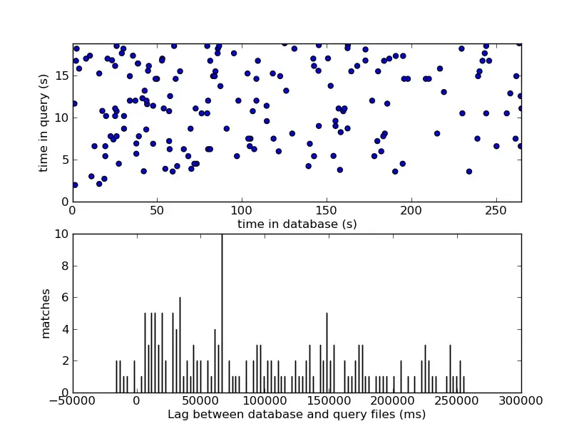
Step 6: Probabilistic Matching and Time-Offset Alignment

When a user triggers Shazam, the app constructs a live constellation map and extracts a set of query hashes using this exact same pipeline. It then queries the central database for matches.

Because individual 32-bit hashes can still collide across an enormous database, a single match proves nothing. The secret sauce of the matching engine lies in coherent time-offset alignment.

For every matching hash found between the query sample and a candidate database track, the engine calculates the temporal offset between the hash's appearance in the user's sample versus its appearance in the studio track:

$\text{offset} = t_{\text{database}} - t_{\text{query}}$

If the query sample genuinely belongs to a specific candidate track, every single surviving hash match from that sample must yield the exact same offset value, because they all preserve their relative spacing from the original recording. Conversely, random collisions from incorrect tracks will generate uncorrelated, chaotic offsets scattered uniformly across the timeline.

The system builds a histogram of these calculated offsets for each candidate track ID and searches for a sharp, undeniable peak in the histogram.

Finding a peak in the histogram is a discrete approximation of identifying a diagonal line on a 2D graph where one axis represents database time ( $t_{\text{database}}$ ) and the other represents query time ( $t_{\text{query}}$ ). If the matched points align perfectly along a 45-degree diagonal line (a slope of $+1$ ), it confirms that both audio sources are progressing at the exact same speed. A significant cluster of points agreeing on a fixed constant offset ( $t_{\text{database}} - t_{\text{query}} = \text{constant}$ ) provides a statistically overwhelming signal that completely cuts through background noise.

A diagram illustrating the time-offset alignment process showing matching hashes converging on a single offset value

The Probability Behind the Magic

Let's make the noise resilience mathematically explicit. Suppose a given spectral peak has a probability $p$ of surviving a noisy recording environment. For a combinatorial hash to be successfully generated, both its anchor and target peaks must survive. The joint probability that a single hash survives is:

$P(\text{hash survives}) = p^2$

While $p^2 < p$ represents a sacrifice in raw survival rate for individual hashes, the trade-off pays off exponentially during lookup. A single surviving paired hash match with proper time alignment is vastly more specific than an isolated peak. The algorithm is structurally designed to require only a small fraction of a song's total hashes to establish an indisputable match, allowing it to recover degraded audio seamlessly.

Technical Glossary

Term	Definition
ADC	Analog-to-Digital Conversion — transforms a continuous sound wave into discrete digital samples
Nyquist Theorem	States that a signal must be sampled at twice its highest frequency to be faithfully reconstructed
FFT	Fast Fourier Transform — an $O(N \log N)$ algorithm for decomposing a signal into frequency components
STFT	Short-Time Fourier Transform — applies FFT over sliding windows to capture time-varying frequency content
Spectrogram	A 2D time-frequency-amplitude representation of an audio signal
Hamming Window	A smooth tapering function applied to each STFT frame to reduce spectral leakage
Spectral Peak	A local maximum in the spectrogram — a point whose amplitude exceeds all neighbors in a defined region
Constellation Map	A sparse set of spectral peak coordinates, forming the basis for fingerprint generation
Combinatorial Hash	A 32-bit hash encoding $(f_{\text{anchor}}, f_{\text{target}}, \Delta t)$ — the core fingerprint unit
Time-Offset Alignment	The matching technique that clusters hash-match offsets to confirm a coherent song identification
Translation Invariance	The property that the fingerprint is independent of where in the song the sample begins

"No Machine Learning" — A Myth-Busting Note for 2026

The classic Avery Wang algorithm is a masterclass in pure, deterministic 1D/2D signal processing and fast hashing. It contains no neural networks, no weights, and no machine learning training models.

However, looking at the architecture from a 2026 perspective, it is worth adding a small modern footnote. While the core matching framework and fingerprint indexing remain anchored to these exact mathematical principles, modern Shazam (operating under Apple's ecosystem) has evolved into a hybrid system. Lightweight, highly optimized Deep Learning models—specifically Convolutional Neural Networks (CNNs)—are now frequently deployed in the initial ingestion phase. These neural models serve as ultra-efficient front-end filters to eliminate extreme external cafe noise, isolate vocals, or perform source separation before the audio enters the constellation mapping phase.

Even with modern AI additions, the core heavy-lifting, matching speed, and ultimate reliability of the system still rest entirely upon the beautiful mathematical foundations laid out more than two decades ago. The next time you tap that button, you are watching the Fourier transform execute something truly timeless.