How Spotify's Recommendation Algorithm Actually Knows Your Soul

If you’ve ever felt that Spotify’s Discover Weekly operates with an almost eerie, clairvoyant precision, you are not alone. You might open the app on a Tuesday evening, let it take over, and suddenly find yourself hit with a track that so perfectly encapsulates your current mood that you start wondering if your phone is listening to you.

The system is not reading your mind, nor is it eavesdropping on your conversations. Matthew Ogle, who led discovery at Spotify during the Discover Weekly era, famously framed the goal as creating “a mixtape from a best friend.” Behind that human-feeling vision, however, lies a system of remarkable mathematical precision.

What feels like digital telepathy is actually the elegant execution of brutal, high-dimensional mathematics. Spotify’s recommendation architecture is a masterclass in modern data science: it does not rely on a single monolithic model, but rather orchestrates an ensemble of distinct machine learning paradigms operating synchronously. Let’s tear down the engine and look at the mathematical architecture under the hood.

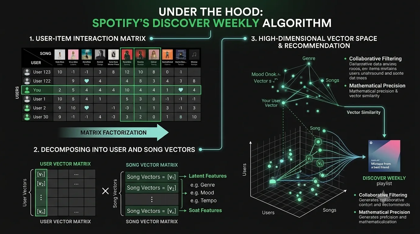Figure 1: The macro orchestration of Spotify’s recommendation engine, demonstrating the pipeline from raw user-item interaction matrix to high-dimensional latent vector embeddings.

---

The Core Architecture: Three Pillars of Extraction

To understand Spotify, we must first differentiate it from deterministic audio-matching algorithms. Shazam, for instance, relies on spectrograms and localized combinatorial hashing to identify a known audio fingerprint against a static database. Spotify, however, solves a fundamentally harder probabilistic problem: predicting future preference based on abstract human behavior it has never directly observed.

To do this, it pulls on three entirely distinct data sources simultaneously — behavior, language, and raw sound.

Pillar 1: Collaborative Filtering via Alternating Least Squares (ALS)

The foundational bedrock of Spotify’s engine is Collaborative Filtering. Instead of analyzing the music itself, it analyzes the metadata of human behavior at a civilizational scale.

Spotify conceptualizes its ecosystem as a massive interaction matrix $R$, where rows represent users ($u$) and columns represent items/songs ($i$). The value in each cell, $r_{ui}$, encodes an implicit signal — a play count, how many times a track was played to completion, whether it was saved, or whether it was skipped in the first 30 seconds. Because users collectively only listen to a tiny fraction of the 100+ million songs available, this matrix is extraordinarily sparse.

The goal is Matrix Factorization: decomposing $R$ into two dense, lower-dimensional matrices — a user matrix $U$ and an item matrix $V$ — such that their dot product approximates the original:

$R \approx U V^T$

Each row of $U$ is a latent feature vector representing a user’s musical taste in some abstract $k$-dimensional space. Each row of $V$ is the corresponding vector for a song. Following standard ML notation, we denote the latent vector for user $u$ as $p_u$ and for item $i$ as $q_i$. Their dot product $p_u^T q_i$ predicts how strongly user $u$ would respond to song $i$.

To learn these vectors at massive scale, Spotify historically utilized the Alternating Least Squares (ALS) algorithm. The objective is to minimize the following weighted loss function:

$J = \min_{P, Q} \sum_{u, i} c_{ui} (r_{ui} - p_u^T q_i)^2 + \lambda (\|p_u\|^2 + \|q_i\|^2)$

Where:

• $r_{ui}$: The observed implicit interaction between user $u$ and item $i$.
• $p_u^T q_i$: The predicted affinity — the dot product of the user and item latent vectors.
• $c_{ui}$: A confidence weight. Since streaming data is implicit (not listening to a song doesn’t necessarily mean disliking it — maybe you just haven’t encountered it), $c_{ui}$ scales the importance of observed interactions proportionally. A song played 50 times receives far more weight in the optimization than a song played once.
• $\lambda$: The L2 regularization parameter to penalize large weights and prevent overfitting.

Because solving for both $U$ and $V$ simultaneously results in a non-convex optimization problem, the ALS algorithm fixes one matrix to solve for the other via linear least squares, then alternates. This trick makes the computation highly parallelizable across distributed clusters — critical when operating on a matrix with 600 million users.

The practical intuition: if your listening behavior closely mirrors a user in Tokyo, the algorithm deduces you are “musical soulmates” and recommends to you the tracks that they love but you haven’t encountered. Your Discover Weekly is, at its core, a curated compilation of what your mathematical nearest neighbors are looping this week.

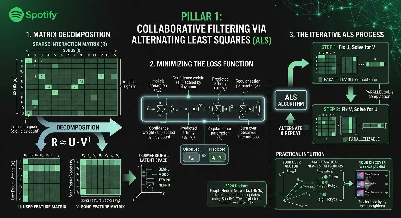Figure 2: The architecture of Spotify’s collaborative filtering framework, illustrating the factorization of the sparse user-item interaction matrix into latent feature vectors, the mathematical loss function optimization, and the iterative execution of the Alternating Least Squares (ALS) algorithm.

Pillar 2: Natural Language Processing — Playlists as Sentences

Collaborative Filtering is powerful, but it suffers from the Cold Start Problem: how do you recommend a track that has zero historical play data? A brand-new upload from an independent artist has no behavioral signal at all. A second, complementary system is needed.

Spotify bridges this gap by turning to the broader cultural internet. Its crawlers continuously scrape web content — music blogs, editorial articles — and most critically, the titles and descriptions of millions of user-generated playlists. Ogle’s famous observation holds here too: the true intelligence of the system “stands on the shoulders of human giants” — the millions of ordinary users who unknowingly label music every time they name a playlist.

The NLP pipeline treats playlists as sentences and songs as words, applying models architecturally similar to Word2Vec (specifically Skip-gram or CBOW variants). By training on the sequence of tracks within playlists, the model is trained to maximize the probability of predicting surrounding tracks given an anchor track — an objective typically optimized via Negative Sampling (a computationally efficient approximation of the full softmax cross-entropy loss). This forces the model to learn dense vector embeddings where songs that co-occur in the same playlists land geometrically close together.

This is the same intuition behind Word2Vec’s famous property: just as “King” − “Man” + “Woman” ≈ “Queen” in word-embedding space, a track that lives between “lo-fi hip hop” and “late night study” playlists will cluster accordingly in music-embedding space.

Once these embeddings are learned, the system evaluates cultural proximity between a candidate track and a user’s preference profile using Cosine Similarity:

$\cos(\theta) = \frac{A \cdot B}{\|A\| \|B\|}$

If thousands of users independently place a track into playlists titled “sad boy hours,” “crying in the rain,” or “2 AM existential crisis,” the vector representation of that song ($A$) drifts measurably closer in the high-dimensional space to the vector representations of those emotional descriptors ($B$). This is exactly why a recommendation hits you at precisely the right moment — the global hivemind has already performed the emotional labeling on Spotify’s behalf.

Spotify refers to these learned representations as “cultural vectors.” They encode not just genre, but mood, context, subculture, and social meaning — dimensions that raw audio analysis simply cannot access.

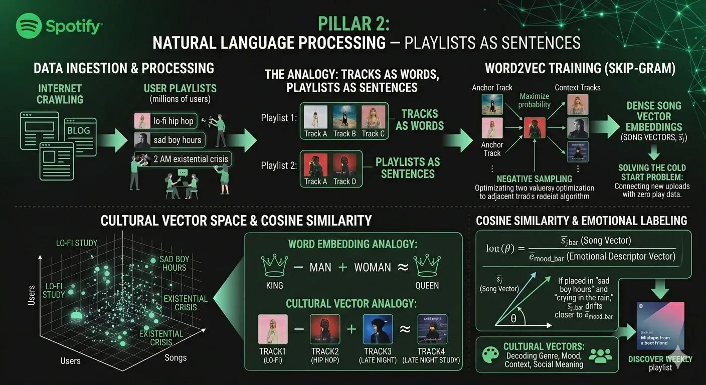Figure 3: The conceptual framework of Spotify’s Natural Language Processing (NLP) pillar, illustrating how user-generated playlists are modeled as semantic sentences via Word2Vec architecture to generate culturally aware song embeddings and calculate emotional proximity.

Pillar 3: Raw Audio Analysis via CNNs

For tracks where both behavioral and textual signals are absent, Spotify’s third pillar takes over: deep acoustic analysis using Convolutional Neural Networks (CNNs) applied to a spectral representation of the audio.

The raw audio waveform is first converted into a Mel-Spectrogram — a two-dimensional representation of the frequency spectrum over time, with frequency bins scaled logarithmically to approximate human auditory perception. The CNN processes this matrix through multiple convolutional layers, learning to detect hierarchical patterns in the sound — from low-level features like transient onsets and tonal stability, up to higher-order qualities like genre texture and emotional register.

The output is a dense feature vector that encodes measurable acoustic characteristics, all normalized to a 0.0–1.0 scale (except loudness, which is measured in dB):

Feature	Scale	What It Captures
Valence	0.0 – 1.0	Musical positiveness. High = euphoric, cheerful. Low = melancholic, tense.
Energy	0.0 – 1.0	Perceptual intensity. Combines dynamic range, loudness, and onset rate.
Danceability	0.0 – 1.0	Rhythmic stability, tempo regularity, and beat strength.
Acousticness	0.0 – 1.0	Confidence that the track is acoustic (natural vs. electronic).
Instrumentalness	0.0 – 1.0	Likelihood of no vocal content. Values above 0.5 are likely instrumental.
Loudness	−60 to 0 dB	Overall average loudness of the track (not playback volume).

By outputting this dense feature vector for any new track, the system can bypass the absence of user data entirely and immediately match the song’s acoustic topology to the preferences of listeners who historically index high on similar vectors. The cold start problem collapses from an insurmountable gap to a simple nearest-neighbor lookup.

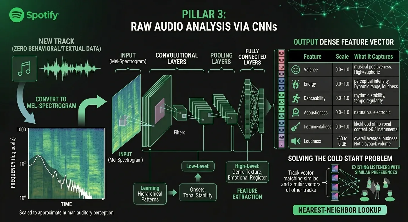Figure 4: The neural network architecture for Spotify’s raw audio analysis, illustrating the extraction pipeline from a log-scaled Mel-Spectrogram through a CNN to generate a dense feature vector of acoustic properties for solving the cold start problem.

---

Discover Weekly: Where the Three Pillars Converge

Discover Weekly is not a single algorithm. It is a product that emerges from the synchronized output of all three pillars above.

Here is a simplified trace of what happens every Monday when your new playlist is assembled:

1. Candidate Generation. The ALS model identifies your nearest neighbors in user-embedding space — listeners whose taste vectors are closest to yours based on recent behavioral signals. From their collective listening history, a pool of candidate tracks is assembled: songs they love that you have not yet heard.

2. Scoring and Re-ranking. Each candidate track is scored against your acoustic profile (from the CNN audio features) and its cultural vector (from the NLP pipeline). A track that appears behaviorally relevant and acoustically consistent and carries cultural descriptors matching your context rises to the top.

3. Novelty Constraint. The system explicitly filters out tracks you have already played or saved. The goal is discovery, not repetition.

4. The 30-Track Limit. Spotify’s product team has consistently stated that 30 tracks is the optimal length for a weekly discovery playlist — long enough to feel comprehensive, short enough to be consumed in a single commute or run. The final ranked list is trimmed to 30, weighted toward higher-confidence recommendations at the top and more exploratory bets at the bottom.

5. Final Re-ranking via BaRT. Before the list is served, the same BaRT (Bandits for Recommendations as Treatments) framework described in the Smart Shuffle section performs a final pass on the ordering. Based on your contextual signals at the moment of opening the app — time of day, listening session history, recent skip rate — it decides whether position #3 on your Monday morning playlist should be a safe, high-confidence choice (exploitation) or a calculated exploratory bet (exploration). The two systems share the same underlying RL engine.

The end result is a playlist that, at its best, feels exactly like a recommendation from a friend who shares your taste but has listened to far more music than you ever could.

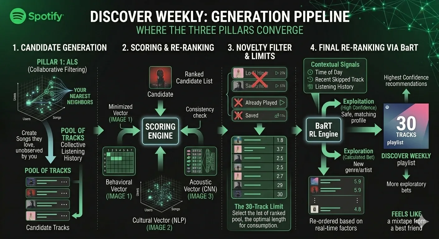Figure 5: The end-to-end Discover Weekly generation pipeline, showing the convergence of collaborative filtering, NLP cultural vectors, and CNN acoustic features into a unified scoring engine, followed by novelty pruning and real-time contextual optimization via the BaRT reinforcement learning framework.

---

The Math of Smart Shuffle: Contextual Bandits

Early in its lifecycle, Spotify utilized a true random generator — the Fisher-Yates shuffle. Statistically, true randomness often yields clustering: it is entirely possible to hear three consecutive songs from the same artist out of a 400-track library. When users encountered this, they complained loudly that the system “wasn’t random.” The perceived randomness failed, even though the mathematical randomness was perfect.

Engineers responded by implementing an algorithm inspired by dithering — a technique borrowed from image processing — that deliberately breaks true randomness to create the perception of fairness by distributing artists evenly across the queue.

Today, standard shuffle has been superseded by Smart Shuffle, an intelligent routing system governed by Reinforcement Learning, specifically an architecture Spotify calls BaRT (Bandits for Recommendations as Treatments).

This is a Contextual Multi-Armed Bandit problem. The algorithm must constantly balance Exploitation (playing tracks it knows you love) with Exploration (injecting unknown tracks to map your evolving taste and prevent you from falling into a “filter bubble”). The class of algorithms driving this is best exemplified by LinUCB (Linear Upper Confidence Bound):

$\text{LinUCB}(a) = \underbrace{ \hat{\theta}_a^T x_{t,a} }_{\text{Exploitation}} + \underbrace{ \alpha \sqrt{ x_{t,a}^T A_a^{-1} x_{t,a} } }_{\text{Exploration}}$

Here is how the algorithm “thinks” in real-time, at every step of your queue:

1. Exploitation ($\hat{\theta}_a^T x_{t,a}$): The predicted reward for choosing track $a$ given your current context vector $x$ — which encodes signals like the time of day, the device type (headphones, car, smart speaker), and recent skip patterns.
2. Exploration Bonus ($\alpha \sqrt{ x_{t,a}^T A_a^{-1} x_{t,a} }$): The statistical uncertainty of that track. Tracks the system has rarely served to users like you in similar contexts receive a mathematically inflated score, encouraging the algorithm to gather more signal about them. $\alpha$ is a tunable hyperparameter controlling the aggressiveness of this exploration.

The feedback loop is direct and brutal: if the algorithm serves an exploratory track and you skip it within 30 seconds, it registers a strong negative reward signal, and the covariance matrix $A_a$ is updated accordingly. If you add the track to your library or turn up the volume, the algorithm has just received confirmation that this contextual gamble paid off. The system learns continuously, adjusting every subsequent decision.

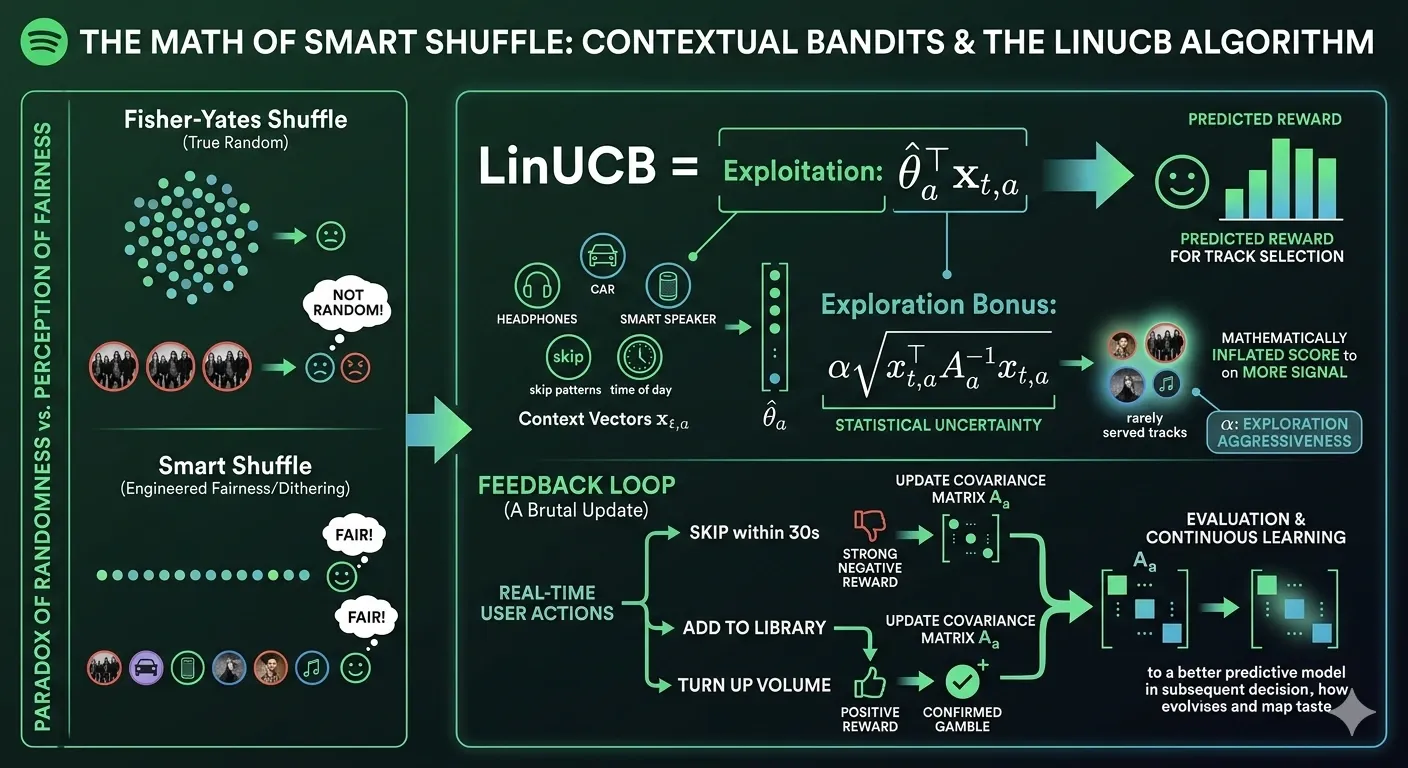Figure 6: The reinforcement learning mechanics of Spotify’s Smart Shuffle feature, contrasting true statistical randomness with perceived fairness and outlining the execution of the LinUCB contextual multi-armed bandit algorithm alongside its continuous real-time user feedback loop.

---

Architectural Shifts: Vector Search and LLMs

The core mathematical theorems governing recommendations have remained stable, but the infrastructure executing them in 2026 has drastically evolved.

Approximate Nearest Neighbors (ANN)

Once users and tracks are represented as vectors, the fundamental operation driving recommendation is a k-Nearest Neighbors (kNN) search: find the $k$ vectors in the database that are closest to a given query vector. Naively computed as dot products across all vectors, this operation scales as $O(n \cdot d)$ per query for $n$ tracks in $d$ dimensions — computationally impossible in real-time for a catalog of 100 million songs.

Spotify’s solution was to build and open-source Annoy (Approximate Nearest Neighbors Oh Yeah), originally built by Erik Bernhardsson in 2013. Annoy partitions the vector space using a forest of random hyperplane trees, allowing approximate nearest-neighbor lookups in $O(\log n)$ time. The trade-off is a small, bounded loss in accuracy — acceptable for recommendations, where a 99.9% optimal result is indistinguishable from a 100% optimal one.

By 2023, Spotify transitioned to their successor library, Voyager, which improved on Annoy’s scalability, memory efficiency, and index build time — critical when the underlying vector database is updated continuously as new user behavior streams in.

The Cognitive Layer: Large Language Models (LLMs)

With the advent of generative AI, the raw mathematical outputs of the recommendation pipeline are now orchestrated by a semantic layer built on LLMs. Features like the AI DJ act as an intelligent translation interface: the LLM interprets unstructured user context — a conversational prompt, an implicit emotional state, the time and location — and translates it into a precise dimensional query against the underlying vector database.

The old systems and the new ones are not in competition. The LLM personalizes the narrative and humanizes the delivery. The matrix factorization, cosine similarity, and LinUCB optimization still perform the heavy lifting of actual music selection. Generative AI is the eloquent front-end; the mathematics is the engine it runs on.

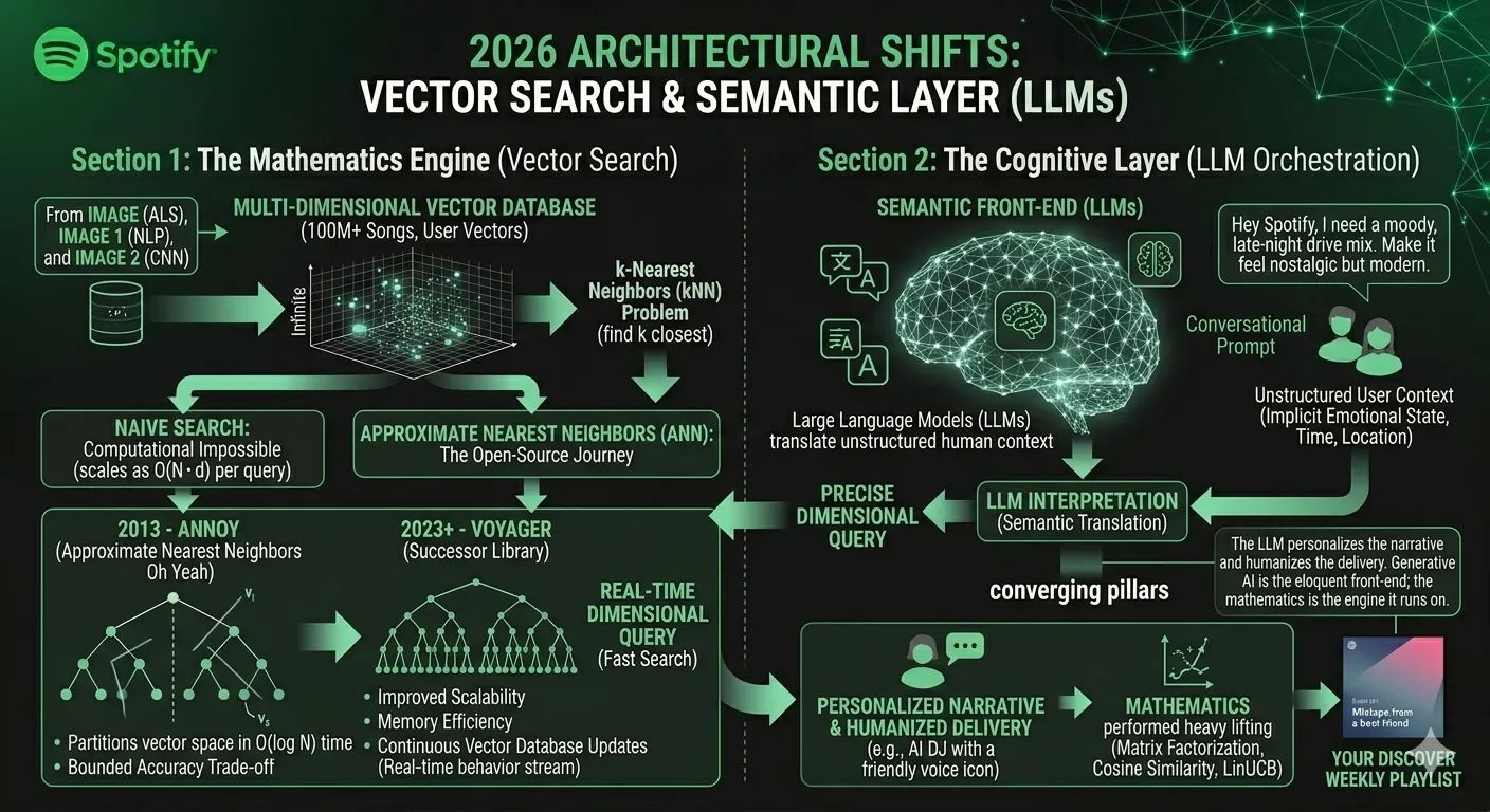Figure 7: Spotify’s unified modern architecture, illustrating the intersection between high-performance approximate nearest neighbors (ANN) vector search libraries like Annoy and Voyager, and the cognitive LLM orchestration layer that translates semantic human context into structured database queries.

---

Technical Glossary

Term	Definition
Collaborative Filtering	Recommendation approach based on shared behavioral patterns between users
Matrix Factorization	Decomposing a sparse user-item matrix into latent factor matrices $U$ and $V$
ALS	Alternating Least Squares — an iterative algorithm for solving matrix factorization
Latent Vector	A dense numerical representation of a user’s or song’s abstract characteristics in $k$-dimensional space
Cold Start Problem	The challenge of recommending items with no historical user interaction data
Word2Vec	A shallow neural network that learns word (or track) embeddings from co-occurrence in sequences
Cultural Vector	A music embedding derived from NLP analysis of playlist titles, articles, and cultural context
Cosine Similarity	A measure of the angle between two vectors; 1.0 = identical direction, 0 = orthogonal
Mel-Spectrogram	A 2D time-frequency representation of audio, frequency-scaled to match human auditory perception
Valence	Audio feature (0.0–1.0) encoding musical positiveness or melancholy
Multi-Armed Bandit	A reinforcement learning paradigm for balancing exploration of unknowns against exploitation of known rewards
LinUCB	Linear Upper Confidence Bound — a contextual bandit algorithm that selects actions based on both predicted reward and uncertainty
ANN / Annoy / Voyager	Approximate Nearest Neighbor libraries for fast vector similarity search in high-dimensional spaces
BaRT	Bandits for Recommendations as Treatments — Spotify’s RL framework for real-time queue personalization

---

Conclusion: A Multi-Dimensional Mirror

Ultimately, Spotify’s recommendation engine is not a mind reader. It is an unblinking, high-frequency mirror — reflecting your own behavioral patterns back at you, amplified by the collective intelligence of over 600 million other listeners worldwide.

Your musical identity within Spotify’s backend is not stored as a list of genres or artists. It is an array of floating-point numbers — a single coordinate floating through an infinite, multi-dimensional space. The algorithm’s ability to find the exact track that matches your Tuesday evening mood is simply the result of billions of continuous matrix multiplications, contextual bandit decisions, and cosine similarity lookups, all converging relentlessly on the point in that vector space where you already live.

The soul it appears to read was always just geometry.